17 Mixed Designs
At a glance
- Question
- Does the change over repeated measurements differ between groups?
- Design
- Two or more independent groups, each participant measured two or more times
- Dependent variable
- Interval or ratio
- Independent variables
- A between-subjects factor (the groups) and a within-subjects factor (the measurements)
- Assumptions
-
- The participants are independent of each other
- DV normally distributed in each group at each measurement
- Equal variances of the groups at each measurement
- Sphericity of the within-subjects factor, the same in all groups
- Null hypothesis
- No main effect of the groups, no main effect of the measurements, and no interaction
- Test statistic
- F for each main effect and for the interaction
- Effect size
- Partial \eta^{2}: .01 small, .06 medium, .14 large
- If conditions fail
-
- The interaction is significant → Simple effects
- Participants have missing measurements → Multilevel model
- Include in the write-up
-
- The design (for example 2 \times 3), and the means at each measurement in each group
- The assumption checks, including Mauchly’s test
- F(df1, df2) = …, p = …, and \eta^{2}_{p} for the interaction and the main effects
- The simple effects
Used when a study has both a between-subjects factor and a within-subjects factor. The participants are divided into groups, as in the one-way ANOVA, and each participant is measured several times or under several conditions, as in the repeated-measures ANOVA. The analysis is called a mixed ANOVA, or a split-plot ANOVA11 The name comes from agricultural experiments, where large plots of land received one treatment and smaller parts of each plot received another..
1 The name comes from agricultural experiments, where large plots of land received one treatment and smaller parts of each plot received another.
The most common mixed design is the pretest-posttest control group design. The participants are randomly assigned to a treatment or a control group and measured before and after the treatment. It solves the main problem of a repeated-measures study without a control group: a change over time in the treatment group can be compared with the change in the control group, which shows what would have happened without the treatment22 See Experimental Versus Non-Experimental Research..
In a mixed design, the question of interest is almost always the interaction: did the groups change differently over time? A main effect of time only shows that the scores changed, on average, in both groups together. A main effect of the group only shows that the groups differed, on average, across all measurements, including the one before the treatment. Neither answers the question the study was designed for.
17.1 The Theory
The mixed ANOVA divides the variability in the same way as the repeated-measures ANOVA, into a part between the participants and a part within the participants. The between-subjects factor is tested in the first part, and the within-subjects factor and the interaction in the second:
- Between the participants. The group effect is tested against the differences between the participants in the same group33 Each participant contributes one value to this test, their mean across the measurements.;
3 Each participant contributes one value to this test, their mean across the measurements.
- Within the participants. The effect of time and the group \times time interaction are tested against the residual variability within the participants, after the individual differences have been removed.
With g groups, k measurements, and N participants, the degrees of freedom are g - 1 and N - g for the group effect, and (k - 1) and (g - 1)(k - 1) for time and the interaction, both tested with (k - 1)(N - g) error degrees of freedom.
Because the two parts have different error terms, the within-subjects effects are usually tested with much more power than the between-subjects effect44 When the measurements of the same participant are strongly related, as they usually are.. This is one more reason why the interaction, a within-subjects effect, is the main test of a mixed design.
4 When the measurements of the same participant are strongly related, as they usually are.
The effect sizes are the partial eta squared of each effect, computed with its own error term and read with the usual guidelines: .01 small, .06 medium, and .14 or more large.
17.2 Assumptions
The mixed ANOVA combines the assumptions of the between-subjects and the within-subjects designs:
- Independence of the participants
- Ensured by the design of the study;
- Violated when the participants influence each other.
- Normality
- Detected using tests of normality of the scores in each group at each measurement;
- Violated when the distributions are strongly skewed or have outliers.
- Homogeneity of variances between the groups, at each measurement
- Detected using Levene’s test at each measurement;
- Violated when the groups have different variances, which is more serious when they also differ in size.
- Sphericity of the within-subjects factor, the same in all groups
- Detected using Mauchly’s test;
- Violated when the variances of the differences between the measurements are not equal. The degrees of freedom of the within-subjects effects are then corrected.
As with the repeated-measures ANOVA, a multilevel model can be used instead. It does not require sphericity and keeps the participants with missing measurements.
17.3 The Study
The counseling center of the repeated-measures chapter wanted to know whether the decrease in stress observed during its mindfulness program was due to the program itself. Forty graduate students who applied to the program were randomly assigned to two groups of 20. The Program group followed the eight-week program right away. The Waitlist group was told that the program was full and that they would follow it in the next semester55 A waitlist control group is a common solution when it would not be ethical to deny the treatment. The control group receives it, but later.. The perceived stress of all students was measured before the program (pre), at its end (post), and two months later (follow-up). The question asked is: Did the stress of the students in the program change differently from the stress of the students on the waitlist? The data set66 Column labels are: student, group, pre, post, and followup. was made up for this example. The first few rows of the data set are shown in Table 17.1.
5 A waitlist control group is a common solution when it would not be ethical to deny the treatment. The control group receives it, but later.
6 Column labels are: student, group, pre, post, and followup.
| Student | Group | Pre | Post | Follow-up |
|---|---|---|---|---|
| 1 | Program | 24 | 21 | 19 |
| 2 | Program | 12 | 13 | 10 |
| 3 | Program | 26 | 20 | 18 |
| 4 | Program | 16 | 14 | 8 |
| 5 | Program | 22 | 17 | 21 |
| 6 | Program | 33 | 22 | 28 |
The design is a 2 (group: program, waitlist, between subjects) \times 3 (time: pre, post, follow-up, within subjects) mixed design.
Hypotheses. The mixed ANOVA tests three pairs of hypotheses. The interaction is the one that answers the question of the study:
- Group \times time interaction. H0: In the population, the change in stress over time is the same in both groups. H1: The change in stress over time differs between the groups.
- Main effect of time. H0: The mean stress, averaged across both groups, is the same at the three measurements. H1: It differs between at least two measurements.
- Main effect of group. H0: The mean stress, averaged across the three measurements, is the same in both groups. H1: It differs between the groups.
Decision criteria. The significance level is set at \alpha = .05 for each effect. H0 is rejected if the p-value is smaller than \alpha. The effect size is \eta^{2}_{p}. If the interaction is significant, it is followed up with simple effects before the main effects are interpreted.
17.3.1 Describing the Data
| Pre | Post | Follow-up | |
|---|---|---|---|
| Program | 25.55 (6.07) | 19.00 (5.46) | 20.10 (5.77) |
| Waitlist | 26.00 (4.44) | 25.35 (6.05) | 24.75 (5.30) |
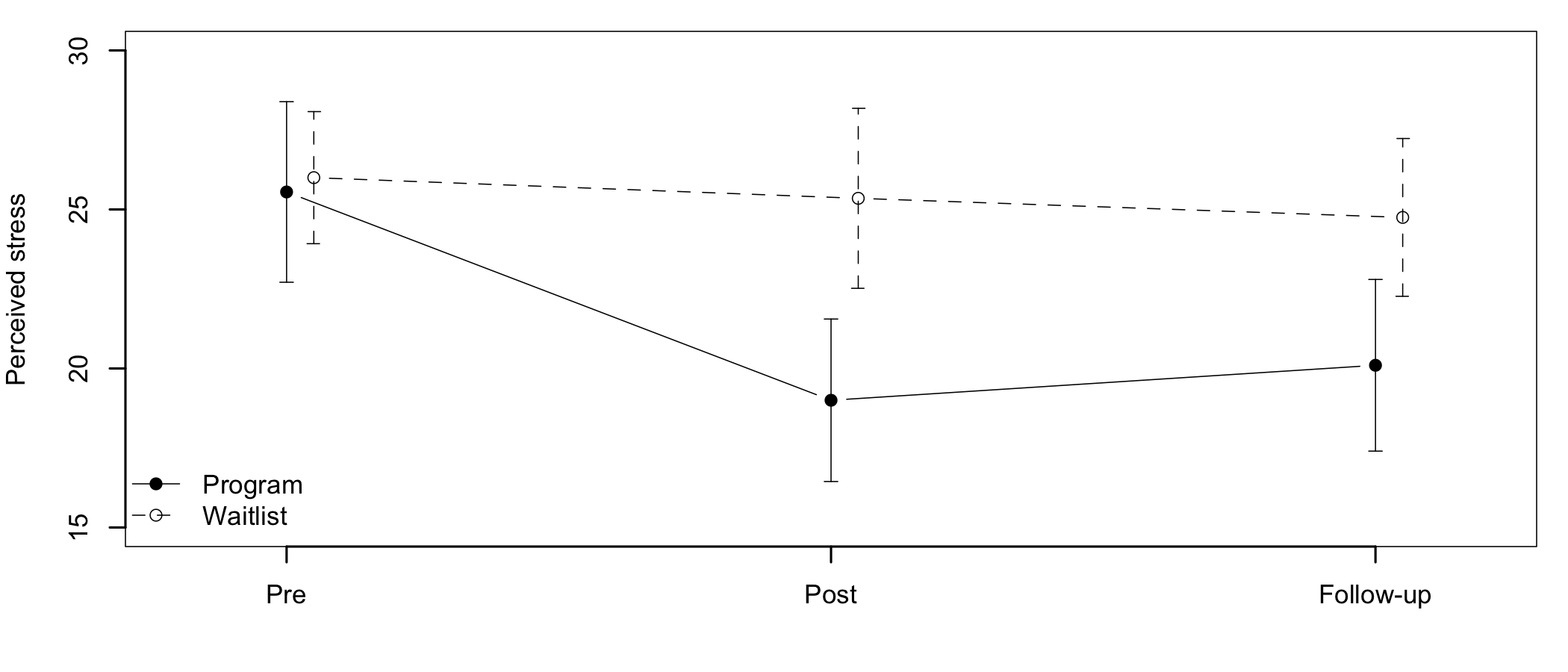
Before the program, the two groups had almost the same level of stress (Table 17.2), as expected from random assignment. At the end of the program, the stress of the students in the program had dropped by 6.6 points, while the stress of the students on the waitlist had barely changed. Two months later, the difference between the groups was still visible. The lines in Figure 17.1 are clearly not parallel.
17.3.2 Checking the Assumptions
The independence of the participants is supported by the design: the students were randomly assigned to the groups and filled in the questionnaire on their own.
               pre      post  followup
Program  0.2828793 0.7888988 0.2805208
Waitlist 0.1557950 0.5098348 0.3523531
pre post followup
0.1517728 0.7860299 0.9043878 - Normality. The Shapiro-Wilk test is not significant in any group at any measurement (p-values between .156 and .789);
- Homogeneity of variances. Levene’s test is not significant at any measurement (p-values between .152 and .904).
Sphericity is tested together with the ANOVA.
17.3.3 The Mixed ANOVA
Univariate Type III Repeated-Measures ANOVA Assuming Sphericity

            Sum Sq num Df Error SS den Df  F value    Pr(>F)
(Intercept)  66035      1  2946.78     38 851.5516 < 2.2e-16 ***
group          437      1  2946.78     38   5.6354   0.02276 *
time           323      2   552.27     76  22.2431 2.485e-08 ***
group:time     184      2   552.27     76  12.6927 1.753e-05 ***
---
Signif. codes:  0 '***' 0.001 '**' 0.01 '*' 0.05 '.' 0.1 ' ' 1


Mauchly Tests for Sphericity

           Test statistic p-value
time               0.9784 0.66768
group:time         0.9784 0.66768


Greenhouse-Geisser and Huynh-Feldt Corrections
 for Departure from Sphericity

            GG eps Pr(>F[GG])
time       0.97886  3.358e-08 ***
group:time 0.97886  2.078e-05 ***
---
Signif. codes:  0 '***' 0.001 '**' 0.01 '*' 0.05 '.' 0.1 ' ' 1

            HF eps   Pr(>F[HF])
time       1.03144 2.484812e-08
group:time 1.03144 1.753329e-05
Mauchly’s test is not significant (p = .668), so the assumption of sphericity is met and the uncorrected tests are used. The rows of the univariate table show the three effects:
- Group \times time: F(2, 76) = 12.69, p < .001, \eta^{2}_{p} = .25;
- Time: F(2, 76) = 22.24, p < .001, \eta^{2}_{p} = .37;
- Group: F(1, 38) = 5.64, p = .023, \eta^{2}_{p} = .13.
Of note is the different number of error degrees of freedom: 38 for the group effect, tested between the participants, and 76 for the two effects tested within the participants.
Decision. The interaction is significant: the change in stress over time was not the same in the two groups. The null hypotheses of the two main effects are also rejected, but they are not interpreted on their own77 The main effect of time, for example, mixes a large change in the program group with almost no change in the waitlist group..
7 The main effect of time, for example, mixes a large change in the program group with almost no change in the waitlist group.
Effect size. The interaction has a large effect, \eta^{2}_{p} = .25.
17.3.4 Simple Effects
The interaction is followed up with simple effects. Two questions are of interest here:
- Did the groups differ at each measurement? They should not differ before the program, and should differ after it if the program works;
- Did the stress change within each group?
The first question is answered with an independent samples t-Test at each measurement, with a Bonferroni correction for the three tests:
                  t df           p
pre      -0.2678025 38 1.000000000
post     -3.4864664 38 0.003756142
followup -2.6550903 38 0.034558425
The groups did not differ significantly before the program (adjusted p = 1.000). The students in the program had significantly lower stress than those on the waitlist at the end of the program, t(38) = 3.49, adjusted p = .004, and two months later, t(38) = 2.66, adjusted p = .035.
The second question is answered with a one-way repeated-measures ANOVA in each group:
                 F df1 df2            p
Program  35.251602   2  38 2.200288e-09
Waitlist  1.034839   2  38 3.650792e-01
The stress of the students in the program changed significantly over time, F(2, 38) = 35.25, p < .001, while the stress of the students on the waitlist did not, F(2, 38) = 1.03, p = .365.
The two sets of simple effects tell the same story: the groups did not differ significantly before the program, only the stress of the students in the program changed significantly, and they were still less stressed than the students on the waitlist two months after the program ended. Because the students were randomly assigned to the groups, the decrease can be attributed to the program.
17.3.5 Reporting the Results
A 2 (group: program, waitlist) × 3 (time: pre, post, follow-up) mixed ANOVA was conducted on the perceived stress of 40 graduate students randomly assigned to an eight-week mindfulness program or to a waitlist. The scores did not depart significantly from normality in any group at any measurement, the variances of the groups did not differ significantly, and the assumption of sphericity was met (Mauchly’s test p = .668). There was a significant group × time interaction, F(2, 76) = 12.69, p < .001, η2p = .25. The groups did not differ significantly before the program (program M = 25.55, waitlist M = 26.00). Stress decreased significantly in the program group, F(2, 38) = 35.25, p < .001, but not in the waitlist group, p = .365, and the students in the program reported lower stress than those on the waitlist at the end of the program (M = 19.00 vs. M = 25.35, Bonferroni-adjusted p = .004) and two months later (M = 20.10 vs. M = 24.75, adjusted p = .035).
17.4 The Multilevel Approach
The same study can be analyzed with a multilevel model, as described in the repeated-measures chapter. The data is first converted to the long format. The model is then built step by step, adding one effect at a time to a baseline model with only the random intercepts of the students, and each model is compared with the previous one.
      Model df      AIC      BIC    logLik   Test   L.Ratio p-value
my.m0     1  3 730.7800 739.1424 -362.3900
my.m1     2  5 705.6761 719.6136 -347.8381 1 vs 2 29.103855  <.0001
my.m2     3  6 702.1448 718.8697 -345.0724 2 vs 3  5.531308  0.0187
my.m3     4  8 683.0892 705.3891 -333.5446 3 vs 4 23.055598  <.0001
Each step improves the model significantly. The last one, which adds the interaction, is the one that answers the question of the study, \chi^{2}(2) = 23.06, p < .001, with the lowest AIC (683.1). The multilevel model confirms the result of the mixed ANOVA.
The changes over time within each group can be compared directly from the final model:
group = Program:
 contrast        estimate    SE df t.ratio p.value
 pre - post          6.55 0.852 76   7.684 <0.0001
 pre - followup      5.45 0.852 76   6.393 <0.0001
 post - followup    -1.10 0.852 76  -1.290  0.6025

group = Waitlist:
 contrast        estimate    SE df t.ratio p.value
 pre - post          0.65 0.852 76   0.763  1.0000
 pre - followup      1.25 0.852 76   1.466  0.4400
 post - followup     0.60 0.852 76   0.704  1.0000

Degrees-of-freedom method: containment
P value adjustment: bonferroni method for 3 tests
In the program group, stress was lower at the end of the program and at follow-up than before it, with no significant change between the end of the program and the follow-up. In the waitlist group, none of the differences is significant.
17.5 Summary
A mixed design combines a between-subjects factor and a within-subjects factor. Its most common form, the pretest-posttest control group design, compares the change over time in a treatment group with the change in a control group. The key result is the interaction. In the mindfulness study, the two groups started at the same level of stress, and only the students who followed the program became less stressed, an effect that lasted two months after the program ended.
Of note is the fact that the control group is what makes the causal conclusion possible. In the repeated-measures study, the decrease in stress could have had other causes. Here, the waitlist group went through the same semester, filled in the same questionnaires, and did not change. The difference between the two groups can therefore be attributed to the program.