19 Chi-Square Test
The Chi-Square Test applies to nominal/categorical variables. It has two forms:
- A one-way classification to estimate how close an observed distribution is to an expected distribution. This type of test is called a goodness-of-fit test.
- A two-way classification to estimate whether two variables from the same population are related or not. This type of test is called a contingency test or test of independence.
Related tests are described with them, for small samples and for the same participants classified twice. Table 19.1 shows which test to use.
| Question and data | Test |
|---|---|
| One variable, compared with an expected distribution | Goodness-of-fit test |
| One variable with two categories, small sample | Binomial test |
| Two variables, enough expected counts | Test of independence |
| Two variables in a 2 \times 2 table, small expected counts | Fisher’s exact test |
| Two variables in a larger table, small expected counts | Simulated p-values or combined categories |
| The same participants classified twice | McNemar’s test |
| The same participants classified three or more times | Cochran’s Q test |
The dataset described below will be used to exemplify both types of analyses. It contains all hospital discharges in New York State in 1993 (12,844 records) for patients admitted with an Acute Myocardial Infarction (heart attack) who did not have surgery. The data is defined as shown in Table 19.2.
| Variable | Explanation |
|---|---|
| age | Patient age in years |
| gender | Patient's gender, coded M for males and F for females |
| diagnosis | Code based on ICD classification |
| drg | Diagnosis Related Group (121 - with complications who did not die; 122 - without complications who did not die; 123 - patients who died) |
| los | Hospital length of stay |
| died | 1 if the patient died in the hospital; 0 if not |
| charges | $ amount of hospital charges |
Let’s take a look at how the data looks like by listing the first few rows of the dataset (Table 19.3).
| diagnosis | gender | drg | died | charges | los | age |
|---|---|---|---|---|---|---|
| 41041 | F | 122 | 0 | 4752.00 | 10 | 79 |
| 41041 | F | 122 | 0 | 3941.00 | 6 | 34 |
| 41091 | F | 122 | 0 | 3657.00 | 5 | 76 |
| 41081 | F | 122 | 0 | 1481.00 | 2 | 80 |
| 41091 | M | 122 | 0 | 1681.00 | 1 | 55 |
| 41091 | M | 121 | 0 | 6378.64 | 9 | 84 |
19.1 Goodness-of-Fit Test
At a glance
- Question
- Does the distribution of one categorical variable match an expected distribution?
- Design
- One group, each participant counted in one category
- Variable
- Nominal, two or more categories
- Assumptions
-
- Independent observations: each participant is counted once
- Expected counts of 5 or more in every category
- Null hypothesis
- The observed counts follow the expected distribution
- Test statistic
- \chi^{2}, with the number of categories - 1 degrees of freedom
- Effect size
- Cohen’s w = \sqrt{\chi^{2}/N}: .10 small, .30 medium, .50 large
- If conditions fail
-
- Two categories and a small sample → Binomial test
- Include in the write-up
-
- The observed counts (or percentages) and the expected distribution
- \chi^{2}(df, N = …) = …, p = …
- Cohen’s w
Looks at a single categorical variable from a population and attempts to assess how close to or consistent with a hypothesized distribution the actual distribution of that variable is.
Hypotheses. The example tests whether the patients are equally distributed across genders:
- Null hypothesis (H0): The data follows the theoretical distribution. Here, the number of male and female patients is the same.
- Alternative hypothesis (H1): The data does not follow the theoretical distribution. The numbers of male and female patients differ.
Decision criteria. The significance level is set at \alpha = .05. The chi-square test has no direction: any departure from the expected counts, in either direction, increases the \chi^{2} statistic. H0 is rejected if the p-value is smaller than \alpha.
Before running the analysis, let’s look at a basic descriptive statistic, frequency analysis.
| Gender | Freq |
|---|---|
| F | 5065 |
| M | 7779 |
Running the chi-square goodness-of-fit test for the gender variable will attempt to test for equal counts in every cell of the design.
    Chi-squared test for given probabilities

data:  table(my.ha$gender)
X-squared = 573.48, df = 1, p-value < 2.2e-16
Decision. With \chi^{2}(1) = 573.48, p < .001, the p-value is smaller than \alpha and H0 is rejected: the numbers of male and female patients are not equal.
Effect size. For a goodness-of-fit test, the effect size is Cohen’s w, computed as w = \sqrt{\chi^{2}/N}. Values around .10 indicate a small effect, .30 a medium effect, and .50 a large effect. Here w = 0.21, a small to medium effect. With 12,844 patients, even a modest imbalance is highly significant, which is why the effect size matters when interpreting the result.
Example of how to write it up:
The null hypothesis stating that patients are equally distributed across genders, \chi^{2}(df = 1) = 573.48, p < .001 is rejected. Therefore, there are significant differences between the expected number of patients for each gender and the observed number.
Observed frequencies can help explain the direction of the relationship for the possible underlying explanation or reason. This explanation can be added to the text if relevant for the study.
19.2 The Binomial Test
At a glance
- Use instead of
- The goodness-of-fit test, when the variable has two categories and the sample is small
- Question
- Does the proportion of a category differ from an expected proportion?
- Design
- One group, each participant counted in one of two categories
- Variable
- Nominal, two categories
- Assumptions
-
- Independent observations: each participant is counted once
- Null hypothesis
- The population proportion equals the expected proportion (\pi = \pi_{0})
- Test statistic
- The number of successes, with its exact binomial probability
- Effect size
- Cohen’s h: 0.2 small, 0.5 medium, 0.8 large
- Include in the write-up
-
- The number of participants, and the number and percentage in the category, with the 95% CI
- The expected proportion
- p = …, and Cohen’s h
When the variable has only two categories, the goodness-of-fit question can also be answered with the binomial test. The binomial distribution gives the exact probability of observing each possible number of “successes”11 The word is used for whichever of the two categories is counted, such as passed, yes, or male. in a given number of trials, when the probability of a success is known. Unlike the chi-square test, the binomial test does not rely on an approximation, and it is the better choice when the sample is small. With large samples, as in the heart attack data, the two tests lead to the same conclusion.
1 The word is used for whichever of the two categories is counted, such as passed, yes, or male.
An example: over the past years, 70% of the students taking a statistics course passed it. This semester the course was redesigned, and 24 of the 28 students passed. The question asked is: Is the pass rate of the redesigned course different from the usual 70%? The numbers were made up for this example.
Hypotheses.
- Null hypothesis (H0): The pass rate of the redesigned course is 70% (\pi = .70).
- Alternative hypothesis (H1): The pass rate of the redesigned course is different from 70% (\pi \neq .70).
Decision criteria. The significance level is set at \alpha = .05, and the test is two-tailed. H0 is rejected if the p-value is smaller than \alpha. The effect size is Cohen’s h, the difference between the observed and the expected proportions after a transformation that makes differences comparable across the whole range from 0 to 122 h = 2 \arcsin \sqrt{p} - 2 \arcsin \sqrt{\pi_{0}}. A difference between .50 and .60 is not the same as a difference between .85 and .95, and the transformation takes this into account.. Values around 0.2 indicate a small effect, 0.5 a medium effect, and 0.8 a large effect.
2 h = 2 \arcsin \sqrt{p} - 2 \arcsin \sqrt{\pi_{0}}. A difference between .50 and .60 is not the same as a difference between .85 and .95, and the transformation takes this into account.
    Exact binomial test

data:  my.passed and my.students
number of successes = 24, number of trials = 28, p-value = 0.09653
alternative hypothesis: true probability of success is not equal to 0.7
95 percent confidence interval:
 0.6733473 0.9596644
sample estimates:
probability of success
             0.8571429
Decision. 86% of the students passed the redesigned course, compared with the usual 70%. However, with p = .097, the p-value is larger than \alpha and H0 cannot be rejected. The 95% confidence interval for the pass rate, from 67% to 96%, includes 70%.
Effect size. h = 0.38, a small to medium effect. A difference of this size cannot be shown with only 28 students: the result does not show that the redesign made no difference, only that one semester is not enough to tell33 See Effect Size and Power for how many students would be needed..
3 See Effect Size and Power for how many students would be needed.
A binomial test compared the pass rate of a redesigned statistics course with the usual pass rate of 70%. Of the 28 students, 24 (86%, 95% CI [67%, 96%]) passed the course. The pass rate was not significantly different from 70%, p = .097, h = 0.38.
19.3 Test of Independence
At a glance
- Question
- Are two categorical variables related?
- Design
- One sample, each participant classified on two variables
- Variables
- Two, nominal
- Assumptions
-
- Independent observations: each participant is counted once, in one cell
- Expected counts of 5 or more; in larger tables, no more than 20% below 5 and none below 1
- Null hypothesis
- The two variables are independent
- Test statistic
- \chi^{2}, with (rows - 1) \times (columns - 1) degrees of freedom
- Effect size
- Phi (\phi) for 2 \times 2 tables, Cramer’s V for larger ones: .10 small, .30 medium, .50 large
- If conditions fail
-
- Small expected counts in a 2 \times 2 table → Fisher’s exact test
- Small expected counts in a larger table → Simulated p-values or combined categories
- The same participants are classified twice → McNemar’s test
- Include in the write-up
-
- The counts or percentages of the table
- \chi^{2}(df, N = …) = …, p = …
- Phi or Cramer’s V, and the cells that differ (standardized residuals)
In this case the Chi-Square Test is used to determine if a significant relationship exists between two categorical variables. The test compares the frequency of each category of one of the variables to the frequency for each of the categories of the other variable.
In this example we will try to find if the number of patient deaths is in some way related to their gender.
Hypotheses.
- Null hypothesis (H0): There is no relationship between gender and the patient dying in the hospital. The two variables are independent.
- Alternative hypothesis (H1): Gender and the patient dying in the hospital are related.
Decision criteria. As before, \alpha = .05, and H0 is rejected if the p-value is smaller than \alpha.
Let’s look at some cell counts first. An idea about how these look like will be useful later when compared with expected cell counts computed from the statistical test.
| 0 | 1 | |
|---|---|---|
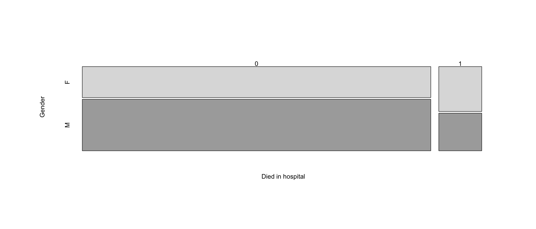
| F | 4298 | 767 |
| M | 7136 | 643 |
Now let’s run the test:
    Pearson's Chi-squared test with Yates' continuity correction

data:  table(my.ha$gender, my.ha$died)
X-squared = 147.76, df = 1, p-value < 2.2e-16
Decision. With \chi^{2}(1) = 147.76, p < .001, the null hypothesis (independence) is rejected and the alternative hypothesis (a relationship between gender and died) is accepted.
Effect size. For a 2 x 2 table, the effect size is the phi coefficient, \phi = \sqrt{\chi^{2}/N}, read with the same guidelines as Cohen’s w. Here \phi = 0.11, a small effect: the relationship is real, but weak.
If the null hypothesis were true, the expected counts are shown in Table 19.6, compared to the observed frequencies shown in Table 19.5.
| 0 | 1 | |
|---|---|---|
| F | 4508.97 | 556.0301 |
| M | 6925.03 | 853.9699 |
A mosaic plot (Figure 19.1) can help visualize the relative cell sizes.
Now let’s look at a chi-square analysis when at least one of the variables has more than two levels. In this case we will be using the drg variable44 The drg (Diagnosis Related Group) has three levels: 121 - with complications who did not die; 122 - without complications who did not die; 123 - patients who died..
4 The drg (Diagnosis Related Group) has three levels: 121 - with complications who did not die; 122 - without complications who did not die; 123 - patients who died.
The cell counts in this case are shown in Table 19.7.
| 121 | 122 | 123 | |
|---|---|---|---|
| F | 2328 | 1970 | 767 |
| M | 3059 | 4077 | 643 |
Hypotheses. H0: there is no relationship between gender and the diagnosis related group (drg). H1: the two variables are related. The decision criteria are the same as above.
Running the test returns the results shown below.
    Pearson's Chi-squared test

data:  table(my.ha$gender, my.ha$drg)
X-squared = 283.43, df = 2, p-value < 2.2e-16
And the mosaic plot is presented in Figure 19.2.
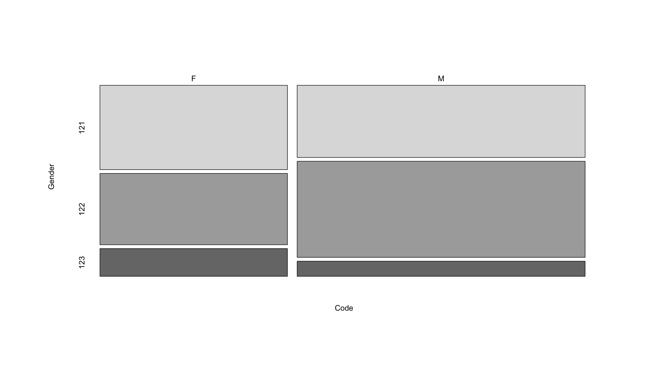
Table 19.8 shows the expected frequencies when the null hypothesis (H0) is true. Compare them with the observed frequencies shown in Table 19.7.
| 121 | 122 | 123 | |
|---|---|---|---|
| F | 2124.35 | 2384.62 | 556.0301 |
| M | 3262.65 | 3662.38 | 853.9699 |
Decision. With \chi^{2}(2) = 283.43, p < .001, H0 is rejected.
Effect size. For tables larger than 2 x 2, the effect size is Cramer’s V, V = \sqrt{\chi^{2}/(N \cdot (k-1))}, where k is the smaller of the number of rows and columns. Here V = 0.15. With k = 2 the same guidelines apply as for phi, so this is a small effect.
Example of how to write it up:
The null hypothesis stating that there is no relationship between gender and diagnosis related group classification, \chi^{2}(df = 2) = 283.43, p < .001 is rejected. Therefore, the differences between the number of males and females in the different diagnosis related group are significant.
19.3.1 Which Cells Differ?
A significant chi-square test shows that the two variables are related, but not where the relationship lies. When one of the variables has more than two categories, the standardized residuals of the cells answer this question. Each one compares the observed count of a cell with its expected count, divided by its standard error:
r_{ij} = \frac{O_{ij} - E_{ij}}{SE_{ij}}
When the two variables are independent, the standardized residuals follow, approximately, the standard normal distribution. A standardized residual larger than 1.96 in absolute value shows a cell with significantly more (positive) or fewer (negative) cases than expected, at \alpha = .05. With many cells, a stricter threshold, such as 2.58 (\alpha = .01) or a Bonferroni-corrected value, reduces the risk of finding differences by chance.
       121    122    123
  F   7.45 -15.00  12.18
  M  -7.45  15.00 -12.18
All six standardized residuals are far beyond 2.58 in absolute value. Women are over-represented among the patients who died (diagnosis related group 123, standardized residual 12.18) and among those with complications (group 121, 7.45), and under-represented among those without complications (group 122, -15.00)55 In a table with two rows, the residuals of the second row are the same values with the opposite sign.. With more than twelve thousand patients, however, even the small effect found above produces large residuals, and the percentages in each column remain the best description of the size of the differences.
5 In a table with two rows, the residuals of the second row are the same values with the opposite sign.
19.4 When the Expected Counts Are Too Small
The chi-square test compares the observed counts with a continuous distribution, the chi-square distribution. The approximation works well only when the expected counts are large enough. The usual rule is that all expected counts should be 5 or more, or, in larger tables, that no more than 20% of them are below 5 and none is below 166 Of note is the fact that the rule concerns the expected counts, not the observed ones. A cell with an observed count of zero is not a problem if its expected count is large enough.. When the rule is not met, the p-value of the test is unreliable77 Statistical software usually warns that the “Chi-squared approximation may be incorrect”.. For a 2 \times 2 table, the solution is Fisher’s exact test, described in the next section. Larger tables have two more solutions, described after it.
6 Of note is the fact that the rule concerns the expected counts, not the observed ones. A cell with an observed count of zero is not a problem if its expected count is large enough.
7 Statistical software usually warns that the “Chi-squared approximation may be incorrect”.
19.5 Fisher’s Exact Test
At a glance
- Use instead of
- The chi-square test of independence, when a 2 \times 2 table has small expected counts
- Question
- Are two dichotomous variables related?
- Design
- One sample, each participant classified on two variables
- Variables
- Two, nominal, two categories each
- Assumptions
-
- Independent observations: each participant is counted once, in one cell
- Null hypothesis
- The two variables are independent
- Test statistic
- The exact probability of the observed table and of all more extreme tables
- Effect size
- The odds ratio, with its 95% CI
- Include in the write-up
-
- The counts of the table
- Why the exact test was used (small expected counts)
- p = …, and the odds ratio with its 95% CI
Used to test the relationship between two variables in a 2 \times 2 table when the expected counts are too small for the chi-square test. A university ran a pilot study of a peer tutoring program for students at risk of failing a course. Twenty students were randomly assigned to receive peer tutoring or not, ten in each group, and the question asked is: Is passing the course related to receiving tutoring? The data set88 Column labels are: student, tutoring, and passed. was made up for this example.
8 Column labels are: student, tutoring, and passed.
          Passed
Tutoring   No Yes
  None      7   3
  Tutoring  2   8
Passed
Tutoring No Yes
None 4.5 5.5
Tutoring 4.5 5.5Hypotheses. H0: Passing the course is independent of receiving tutoring. H1: Passing the course is related to receiving tutoring.
Decision criteria. \alpha = .05. Two of the four expected counts are below 5, so the chi-square test cannot be used. Fisher’s exact test computes the exact probability of the observed table, and of all tables more extreme than it, given the row and column totals. It does not rely on an approximation and can be used with any sample size. H0 is rejected if its p-value is smaller than \alpha. The effect size is the odds ratio, the odds of passing with tutoring divided by the odds of passing without it.
    Fisher's Exact Test for Count Data

data:  my.pt
p-value = 0.06978
alternative hypothesis: true odds ratio is not equal to 1
95 percent confidence interval:
   0.8821175 127.0558418
sample estimates:
odds ratio
  8.153063
Decision. Fisher’s exact test is not significant, p = .070. H0 cannot be rejected: with only 20 students, the pilot study does not show that tutoring is related to passing the course.
Effect size. The estimated odds ratio is 8.15, but its 95% confidence interval runs from 0.88 to 127.06 and includes 1 (no relationship). The effect could be large, but the sample is too small to estimate it with any precision.
Of note is what would have happened with the wrong test. The chi-square test without any correction gives \chi^{2}(1) = 5.05, p = .025, a significant result. With small expected counts, the chi-square approximation is too liberal: it rejects H0 more often than \alpha. Yates’ continuity correction, which is often applied to 2 \times 2 tables by default, makes the test more conservative, \chi^{2}(1) = 3.23, p = .072, but Fisher’s exact test is the better choice when the expected counts are small. For a pilot study, the right conclusion is that a larger study is needed, not that tutoring works99 See Effect Size and Power for how the sample size of the larger study can be planned..
9 See Effect Size and Power for how the sample size of the larger study can be planned.
19.6 Simulated p-Values and Combining Categories
In tables larger than 2 \times 2, two more solutions are available. As an example, 45 students taking the same course were asked where they usually study: in the Library, at Home, or in a Cafe. The question asked is: Is the preferred study location related to the year of study? The data set1010 Column labels are: student, year, and location. was made up for this example.
10 Column labels are: student, year, and location.
            Location
Year         Library Home Cafe
  First-year      10    8    2
  Sophomore        6    8    1
  Junior           0    8    2
Location
Year Library Home Cafe
First-year 7.11 10.67 2.22
Sophomore 5.33 8.00 1.67
Junior 3.56 5.33 1.11Of the 9 expected counts, 4 are below 5, most of them in the Cafe column, chosen by few students.
The first solution is to compute the p-value by simulation. Thousands of tables with the same row and column totals are generated at random, as if H0 were true, and the p-value is the proportion of these tables with a chi-square statistic at least as large as the observed one. Like Fisher’s exact test, the simulation does not rely on the chi-square approximation.
    Pearson's Chi-squared test with simulated p-value (based on 10000
    replicates)

data:  my.sl
X-squared = 7.8125, df = NA, p-value = 0.09879
With a simulated p = .099, the relationship between the year of study and the study location is not significant.
The second solution is to combine categories until the expected counts are large enough. The combination must make sense for the question asked, and it changes the question. Here, the library is the only place on campus designed for studying, and combining Home and Cafe into a single Elsewhere category turns the question into: Is studying in the library related to the year of study?
            Location
Year         Library Elsewhere
  First-year    7.11     12.89
  Sophomore     5.33      9.67
  Junior        3.56      6.44
    Pearson's Chi-squared test

data:  my.sl2
X-squared = 7.4677, df = 2, p-value = 0.0239
Of the six expected counts, 1 is now below 5, and none is below 1, which meets the 20% rule. The test is significant, \chi^{2}(2) = 7.47, p = .024, Cramer’s V = 0.41: 50% of the first-year students study mostly in the library, compared with 40% of the sophomores and 0% of the juniors.
The two solutions lead to different conclusions because they answer different questions. The simulated test asks whether the three locations are chosen differently by the three years, the combined test whether the library is. The choice between them, and the way categories are combined, must be decided before looking at the results. Trying several combinations until one of them is significant inflates the risk of a Type I error.
Here is an example of how to write up the result of the combined test:
Because several expected counts were below 5, the home and cafe categories were combined. A chi-square test of independence showed that studying in the library was related to the year of study, χ2(2, N = 45) = 7.47, p = .024, V = .41. First-year students (50%) studied mostly in the library more often than sophomores (40%) and juniors (0%).
19.7 McNemar’s Test
At a glance
- Use instead of
- The chi-square test of independence, when the same participants are classified twice
- Question
- Did the proportion of participants in a category change between two measurements?
- Design
- One group, classified twice (before and after, or under two conditions)
- Variable
- Nominal, two categories
- Assumptions
-
- Paired observations: the same participants, or matched pairs
- Each participant, or pair, is independent of the others
- Null hypothesis
- Changes in the two directions are equally likely, so the proportion does not change
- Test statistic
- \chi^{2}, with one degree of freedom
- Effect size
- The change in the proportion, and the odds ratio of the two kinds of change
- If conditions fail
-
- Fewer than about 25 participants changed → the exact version, a binomial test of the changes
- Include in the write-up
-
- The number of participants, and the proportion in the category at each measurement
- The number of participants who changed in each direction
- \chi^{2}(1, N = …) = …, p = …
All the tests above assume that the observations are independent: each participant is counted once, in one cell of the table. When the same participants are classified twice, for example before and after a treatment, the observations are paired, and the chi-square test of independence cannot be used. McNemar’s test is the test for such data. It is to categorical variables what the paired samples t-Test is to interval and ratio variables.
An example: before a two-hour workshop, 60 students were asked “Can you read the results table of a statistical test?” and answered Yes or No. After the workshop, they were asked the same question again. The question asked is: Did the proportion of students who answer Yes change after the workshop? The data set1111 Column labels are: student, before, and after. was made up for this example.
11 Column labels are: student, before, and after.
      After
Before Yes No
   Yes  14  5
   No   21 20
Each student appears once in the table, in the row of their first answer and the column of their second. The students on the diagonal, 14 who answered Yes both times and 20 who answered No both times, did not change. McNemar’s test uses only the students who changed: the 21 who went from No to Yes, and the 5 who went from Yes to No. If the workshop made no difference, changes in the two directions would be equally likely.
Hypotheses.
- Null hypothesis (H0): In the population, the proportion of students who answer Yes is the same before and after the workshop. Changes from No to Yes and from Yes to No are equally likely.
- Alternative hypothesis (H1): In the population, the proportion of students who answer Yes changes after the workshop.
Decision criteria. The significance level is set at \alpha = .05. The test statistic compares the two kinds of change, b (from Yes to No) and c (from No to Yes), and follows a chi-square distribution with one degree of freedom1212 The 1 subtracted from the difference is a continuity correction, which makes the approximation more accurate.:
12 The 1 subtracted from the difference is a continuity correction, which makes the approximation more accurate.
\chi^{2} = \frac{(|b - c| - 1)^{2}}{b + c} = \frac{(|5 - 21| - 1)^{2}}{5 + 21} = 8.65
H0 is rejected if the p-value is smaller than \alpha. When fewer than about 25 students changed, the exact version of the test should be used instead: a binomial test of the number of changes from No to Yes, out of all changes, with an expected probability of .5. The effect size is the change in the proportion of Yes answers, together with the odds ratio of the two kinds of change, c/b.
    McNemar's Chi-squared test with continuity correction

data:  my.ws
McNemar's chi-squared = 8.6538, df = 1, p-value = 0.003264
Decision. With \chi^{2}(1) = 8.65, p = .003, H0 is rejected: the proportion of students who answer Yes changed after the workshop.
Effect size. The proportion of Yes answers rose from 32% before the workshop to 58% after it. Of the 26 students who changed their answer, 21 changed in favor of Yes: the odds of changing toward Yes rather than toward No are 4.20 to 1.
Of note is the fact that the chi-square test of independence, run on the same table, would answer a different question: whether the answers before and after are related, which they almost always are, because they come from the same students. McNemar’s test asks whether they changed. As with the paired samples t-Test, a change in a single group does not show that the workshop caused it.
McNemar’s test compared the answers of 60 students who were asked, before and after a two-hour workshop, whether they could read the results table of a statistical test. The proportion of students who answered yes increased from 32% to 58%, χ2(1, N = 60) = 8.65, p = .003. Of the 26 students who changed their answer, 21 changed from no to yes and 5 from yes to no.
19.8 Summary
The chi-square tests compare observed counts with the counts expected under a hypothesis: a theoretical distribution for the goodness-of-fit test, and independence for the test of independence. A significant result is followed up with the standardized residuals, which show the cells that depart from the expectation. The tests rely on an approximation that requires large enough expected counts. When they are too small, Fisher’s exact test, simulated p-values, or meaningfully combined categories should be used instead. With large samples, as in the heart attack data, even weak relationships are significant, and the effect size, phi or Cramer’s V, tells whether they matter. For a variable with two categories, the binomial test gives an exact goodness-of-fit test, which is preferred in small samples. When the same participants are classified twice, the observations are not independent, and McNemar’s test replaces the test of independence.